
Predicting Dwelling Occupancy: An Analysis Based on Income, Education, and Marital Status
Predicting Dwelling Occupancy: An Analysis Based on Income, Education, and Marital Status
Abstract:
The aim of this study to predict if the dwelling is occupied by the owner or rental based on several key factors: income, education, and marital status. To classify the dataset, we have used the Support Vector Machine technique with RBF and polynomial kernel. The model potentially can be used in assisting policymakers, real estate professionals, and other stakeholders in understanding the housing occupancy patterns. The analysis also incorporates costs associated with running the property, such as gas, fuel, and electricity.
Introduction:
The purpose of this research is to apply a methodology to forecast whether a property is owned or rented, as well as to discover the features that have a significant influence in determining house ownership status. The data was obtained by IPUMS USA, which acquired the information through the US Census. The dataset includes factors linked to people and their living situations, such as age, income, and education level. It also takes into account home characteristics like power costs, year of construct, and population density in the surrounding area. We used support vector machine to classify the data, as well as other extensions of the SVM model using rbf and polynomial kernel, and cross validated the models, achieving an accuracy of 86 percent in categorizing the data.
Theoretical Background:
Support Vector Machine (SVM) is a maximal margin classifier that requires a linear boundary to separate classes. It can handle classification and regression problems. The Support Vector Classifier (SVC) is an extension that uses a kernel function to handle a wider range of cases. The support vector machine uses hyperplane to separate the classes. A hyperplane in a p-dimensional space is a flat subspace of dimension of p-1. It can be visualized as a line in two dimensions or a plane in three dimensions. Although it may be challenging to visualize a hyperplane in spaces with more than three dimensions, the concept of a flat subspace with a dimension of p-1 still holds. A hyperplane is in p-dimension is defined by the equation: β0 + β1X1 + β2X2 + · · · + βpXp = 0 A point X in p-dimensional space lies on the hyperplane if it satisfies the equation. If β0 + β1X1 + β2X2 + · · · + βpXp is greater than zero, X is on one side of the hyperplane, and if it is less than zero, X is on the other side. However, if data is perfectly separated by the hyperplane, then there can exist infinite number of hyperplanes which separates the data as can be seen by the Figure 1.a. Hence, it becomes important to pick which hyperplane to choose to separate the data which gives rise to concept of the maximal margin hyperplane. It is the optimal hyperplane separating two classes. The SVM uses the principle of maximizing the distance between nearest data points from the hyper plane from either class. The distance between the hyperplane and the point is called as margin as shown in Figure 1.b. The more the distance between the margin the better the model is. The nearest data points to the hyperplane are called as the support vectors. The decision of finding the hyperplane is fully governed by subset of the training samples and the support vectors. Therefore, the support vectors play a critical role in determining the position of the hyperplane, and their removal could potentially change the location of the hyperplane. They are very critical in determining the optimal hyperplane.
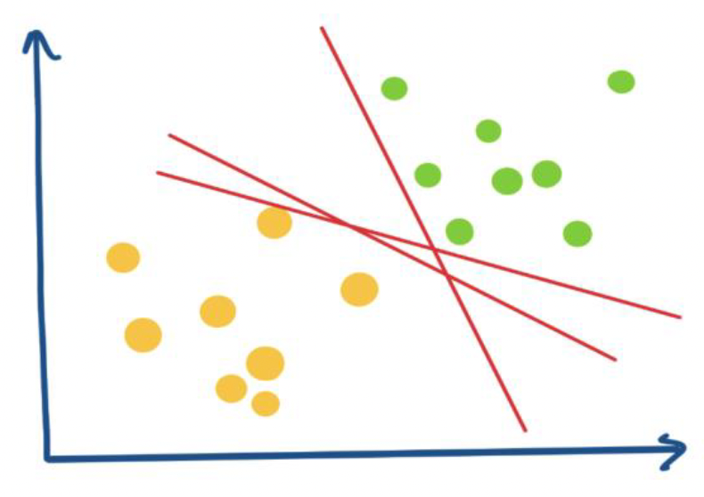 Figure 1.a: Infinite plane to separate the data.
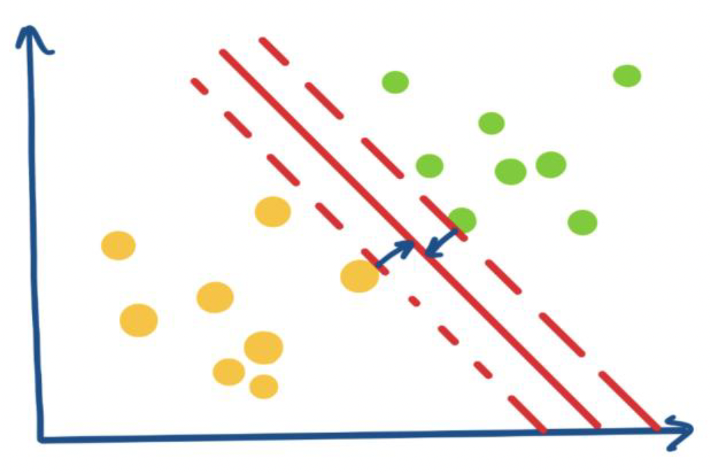 Figure 1.b Distance between two classes: margin
SVM’s kernel hyperparameter is crucial for model performance, with options including linear, polynomial, and radial kernels. Tuning these hyperparameters can have a significant impact on model accuracy. SVM works best in high-dimensional spaces and with linearly separable data but can struggle with large datasets due to slow training time as we need to calculation which involved find optimal distance. If the data is not linear separable then the Hard Margin SVM won’t work since, we won’t be able to find the optimal hyperplane which separates two classes hence we can adjust the cost parameter or choose a different kernel. The polynomial kernel is a type of kernel used in Support Vector Machines (SVMs) that is useful for separating data that is not linearly separable but can be separated by a polynomial function. The basic idea is to transform the input data into a higher-dimensional space where it can be linearly separated, and then build a linear model on top of it to separate the classes. The kernel function used in polynomial kernel SVM is defined as K (x, y) = (x * y + c) ^ d, where x and y are input feature vectors, c is a constant, and d is the degree of the polynomial. When d is 1, the polynomial kernel is the same as the linear kernel, and when d is higher, the kernel function maps the data into a higher-dimensional space, making it easier to separate the classes. The value of c is a regularization parameter that controls the tradeoff between the model’s ability to fit the training data and its ability to generalize to new data. The degree parameter controls the complexity of the polynomial function used to separate the data. If the degree is too low, the model may not be able to separate the data effectively, while if the degree is too high, the model may overfit the data and perform poorly on new data. Tuning these hyperparameters is important for achieving good performance with polynomial kernel SVMs. The RBF kernel (Radial Basis Function) is a popular kernel used in SVM (Support Vector Machine) for non-linear classification problems. It works by creating a “bump” or “hill” in the transformed data space around each data point, where the height of the bump depends on how important that data point is in determining the class separation. The RBF kernel essentially maps the input data into a higher-dimensional space where it is easier to separate the classes. It does this by measuring the distance between each data point and creating a Gaussian-shaped bump around it. The size of the bump is controlled by a hyperparameter called gamma, and it determines the smoothness of the boundary between the classes. After transforming the data into this higher-dimensional space, the SVM algorithm finds a way to draw a separating boundary through the “valleys” between the bumps, which effectively separates the classes. This boundary is called the hyperplane and is defined by a set of weights assigned to each data point. In summary, the RBF kernel creates a non-linear decision boundary by transforming the data into a higher-dimensional space and creating Gaussian-shaped bumps around each data point. The SVM algorithm then finds a hyperplane that separates the classes by passing through the “valleys” between the bumps.
Methodology:
The aim of this research was to predict if the housing is occupied by owner or rented. The dataset provided a unique challenge as each row represented a dwelling with multiple occupants living in a same home. Please refer to the screenshot which shows how the household data is defined. SERIAL provides a unique identification number for each household in a dwelling and we can see that there are multiple records. 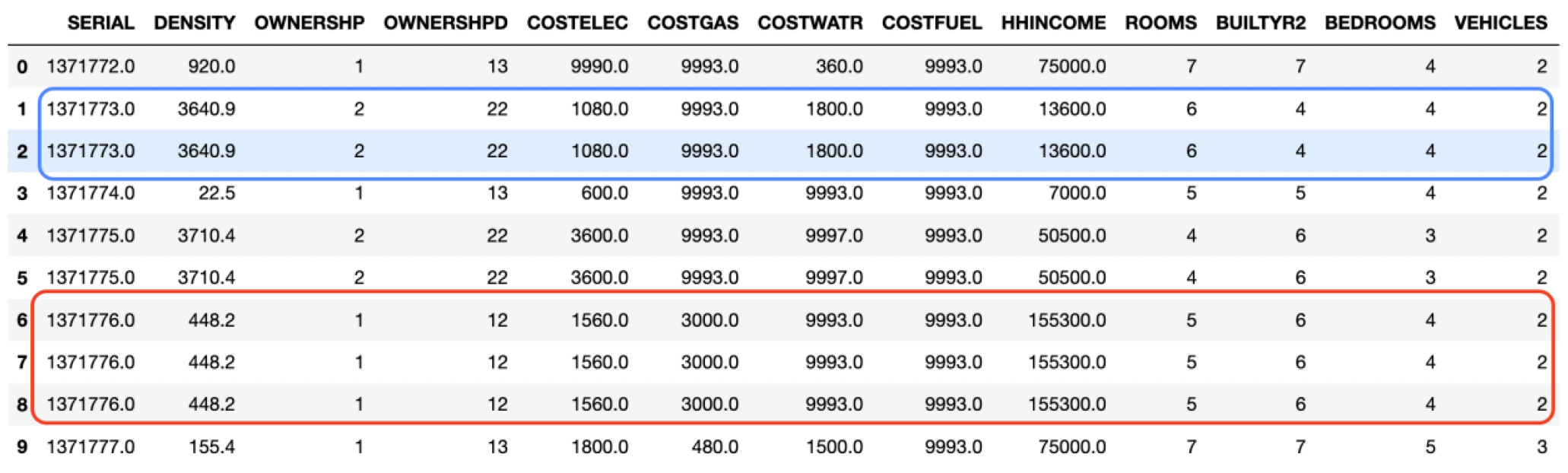
Figure 2: Duplicated rows in the data (3 out of 23 columns) had unique values.
Further analysis revealed only 35% (8 out of 23 columns) of the columns had unique values. It’s important to look into these features (Table 1) and see how we want to aggregate the data since; rest of the data is redundant and does not provide any new information. It’s important to deal with the how we are going to deal with the age and marital status column in our dataset. In our dataset, we have taken the maximum value of age, marital status, and average of income since, that’s going to derive the decision if the house is rented or owned by an individual. The reasoning for selecting the maximum value of age is since children cannot own a house. Therefore, it is more appropriate to choose the highest possible value of age.
| Column | Description |
| PERNUM | Consecutive household member numbering system in IPUMS dataset. |
| PERWT | Indicates a person’s representation in IPUMS sample population |
| AGE | The person’s age in years as of the last birthday |
| MARST | Each person’s current marital status |
| BIRTHYR | Person’s year of birth. |
| EDUC | Respondents’ educational attainment, as measured by the highest year of school or degree completed |
| EDUCD | Respondents’ educational attainment, as measured by the highest year of school or degree completed |
| INCTOT | Respondent’s total pre-tax personal income or losses |
Table 1: displays the columns that contained unique values.
We have also removed the features like Birthyear, education and highest income since they are highly correlated with age, educational code and income. This helps in removing the redundancy in the data. Once we aggregated the data based on columns having the same value, we observed a significant reduction of 47.47% (from 75388 rows to 35802) in the data volume. This led to a substantial improvement in performance. Next, we addressed the data columns that included the cost of electricity, water, and fuel. The predictors associated with these records had a particular code 9999, 9993 that indicated whether there was no cost or if these expenses were already included in the rent. It was crucial to replace these values with 0 in these cases. We used SVM for classification tasks to accurately identify the houses, employing a variety of demographic and environmental parameters as predictors such as age, education level, family income, and cost of maintaining a property. We used cross-validation techniques to assess the performance of our model. Later, we expanded our model to include the rbf kernel and polynomial kernel with varying cost, gamma, and polynomial degree values. We found that even after training the model with such hyperparameters, the results were comparable to what we were achieving with the linear SVM model. As a result, I chose the linear model as the final model because it required less computational effort to achieve the comparable outcomes. In summary, our process includes recognizing and addressing outliers, considering how to aggregate the data based on the unique features, and then training the SVM model and evaluating its performance on test dataset.
Computational Results:
To build the model which classify the dwelling as rented or owned. I have used various variables like income, marital status, education and the cost which involves running the house like money spent on gas, electricity and fuel. We have achieved 85% accuracy in classifying the dwelling and have tried various models in classifying the dwellings. We have used linear, rbf and polynomial kernels to train the machine learning model. We cross validated the model using cost, gamma, and degree hyperparameters. It was observed that the model was giving almost similar accuracy with rbf and linear kernel. Hence, it’s advised to use the linear kernel since it is more robust and less prone to overfitting. We can see that in the table 2. | Kernel | Cost | Gamma | Degree | Cross validation error | Accuracy rate | | Linear | 1 | - | - | 16% | 83.5% | | Radial | 100 | 6 | - | 15% | 84.5 % | | Poloynomial | 10 | - | 4 | 14% | 97.72 % |
Table 2: SVM computational model output with hyperparameters.
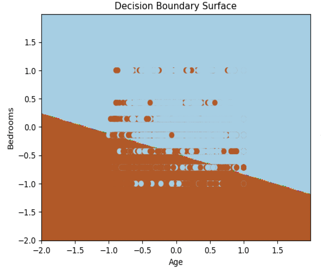 Fig 3.a: Decision Boundary Surface: Linear
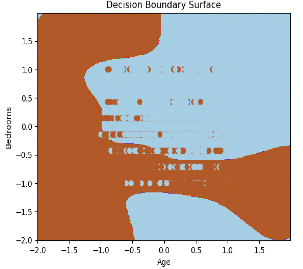 Fig 3.b: Decision Boundary Surface: RBF Kernel
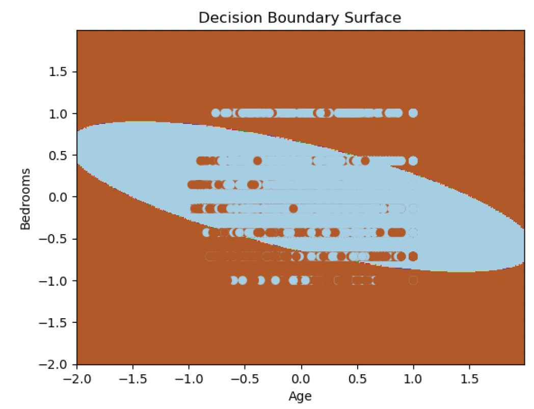 Fig 3.c: Decision Boundary Surface: Polynomial Kernel
The model was working well on the test dataset as well. I got the same accuracy and error on the test set as I was getting on training set. It conveys that the model was not overfitting. We can see the decision boundary in Figure 3 for all the three models along with the confusion matrix on Figure 4 and see how model is performing. Since, we can’t plot the higher dimensions on 2D, we will plot the data using Age and Rooms feature from the dataset and then see how the decision boundary is. We can see that somehow the rbf kernel boundary might be overfitting the data.
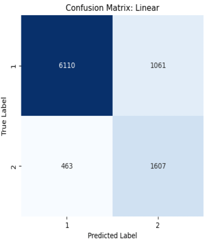 Fig 4.a: Confusion Matrix Linear
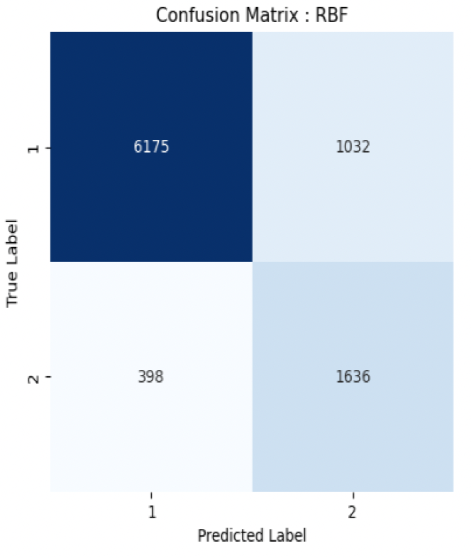 Fig 4.b: Confusion Matrix RBF
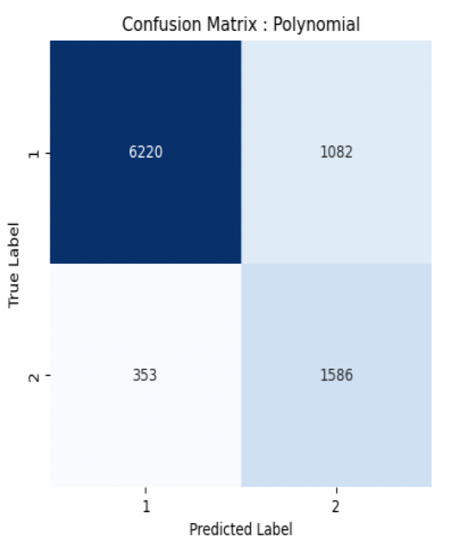 Fig 4.c: Confusion Matrix Polynomial
The computation result shows the precision, recall, and F1-score of a binary classification model’s performance on a dataset can predict class “1: Owned” with 85% precision and identify 93% of actual class “1” instances, while predicting class “2: rented” with 78% precision and identifying 60% of actual class “2” instances. The overall weighted average precision, recall, and F1-score are 0.83, 0.84, and 0.83, respectively, indicating that the model’s predictions are correct 83% of the time and it can identify 84% of all instances. I certainly believe that there’s still room for the improvement and if we have more features and data then we can perform and tune our model better to classify the data. We could have also tried some more advance techniques to train the data and achieved the higher accuracy.
Discussion:
It is worth noting that the IPUMS USA dataset includes a vast array of data that can be used to answer many more questions related to the dwelling’s ownership. Our study concentrated specifically on the people’s income, age, and education, which was just one component of the data. Nonetheless, our findings provide valuable insights into knowing that which variables are important to determine if people will own the house or not. Our findings show that these factors have a considerable impact on a person’s likelihood of purchasing a home later in life. The data may have been further studied by answering questions based on parental education status and income and determining whether or not the child will buy their own home later in life. Apart from income and education, the study intended to classify whether the space is owned or rented based on several aspects such as the cost of maintaining the space such as electricity, fuel, and gas. According to the findings, income and education play a crucial effect in deciding who will own the house. On test results, the SVM model attained an accuracy of 86%, suggesting its usefulness in identifying the residence. Furthermore, adding rbf or polynomial kernel had no effect on the model’s accuracy. However, the study had limitations such as the cross-sectional nature of the data, which limits the ability to infer causality, and self-reported data because the data was too correlated, resulting in data loss of nearly 50%. We didn’t have many features to work with, such as bedrooms and rooms, which were significantly associated. Other examples include the relationship between income and highest income, as well as education and education code. Furthermore, the sample size of the dataset was relatively small, which may limit the generalizability of findings to a larger population.
Conclusions:
Our study aimed to classify the dwelling using Support Vector Machine models and extension of those models’ using RBF and polynomial kernel. We utilized data from the by IPUMS USA, which acquired the information through the US Census and found that the models were able to achieve impressive accuracies. For the binary classification problem, the SVM after aggregating the data achieved an accuracy of 85.09%. These findings imply that support vector machines are good tools for predicting whether a person would purchase or rent a home. The models’ performance is encouraging and highlights their potential in aiding real estate agent, policy makers to device a policy which help the company as well as any individual. Overall, our study contributes to the existing body of literature on the use of Support Vector Machine models with extension of kernels in classifying the dwellings. References:
IPUMS USA. dataset (n.d.). Retrieved from https://usa.ipums.org/usa/index.shtml